Tutorial 1
Contents
Tutorial 1#
In this tutorial we are going to walk through each step of the DS4FNP stack.
Data Stacks For Fun & Nonprofits is a series of articles and tutorials aimed towards designing and implementing a modern data stack using open source and open core components. The DS4FNP stack is intended to be accessible enough for education purposes (both in terms of costs and being laptop-deployable), but suitably scalable as a mature analytics architecture for organizations of all sizes.
In a previous article, I described and outlined the rationale behind a locally deployable stack composed of Postgres, Meltano, Airflow, dbt, and Apache Superset. The Postgres database can be swapped out for other database engines such as SQLite and MySQL with few significant implications. This setup allows us to work with a full data stack in a local environment, and then when we are ready to scale to a cloud hosted data warehouse like BigQuery or Snowflake, doing so is a simple matter of switching some configuration files.
We’re now ready for a hands-on tutorial demonstrating how to setup each component of the stack and some example content. We’re going to walk through the setup of each component in the stack, extract and load data into a data warehouse (ok, really just a local database for now), and design some basic analytics dashboards.
Finding some data!#
Before we get started, we need to come up with some kind of purpose or scenario to motivate our selection of data sources and objectives. This is always the most difficult part of designing tutorials for such diverse potential use cases, as you want to try to present something relevant to all cases. I think that an ideal scenario would be one that involves continuously generated data, such as sports statistics or server logs, as these would allow us to think in terms of regularly scheduled workflows and longitudinal plots. However, in the interest of learning to walk before we run, let’s save those scenarios for a future tutorial and for now focus on some slower moving data.
The past few months have been occupied with news about the 2020 US Elections, and finalized returns are now being made available from the usual sources, so this seems like a timely and suitable theme to go with. From an analytical perspective, let’s set our interests on comparing recent and historical election results.
Perhaps unsurprisingly, it turns out that data on US elections is incredibly decentralized, not always obvious where to find or how to access, and lacking any kind of common standards. There are a few public institutions and academic researchers who bravely collect and publish some datasets, many of which I have begun to catalog and curate at https://github.com/andrewcstewart/awesome-democracy-data. If you are interested in data related to elections, electoral reforms, and democratic political systems, I encourage you to take a look!
The primary data source we will use for this tutorial is from the MIT Election Data + Science Lab. Specifically, we are interested in collecting historical US elections results for the House of Representatives, the Senate, and Presidential candidates in the Electoral College.
Collecting data with Meltano#
You will need the following for this tutorial:
Download and install PostgreSQL.
You may to use a SQL client: I recommend TablePlus or pgcli.
Most of the components in the stack depend on Python3.
I also recommend using an IDE, such as VS Code (along with the vscode-dbt extension.)
Let’s begin! If you just want to follow along, all the code/configuration generated during this tutorial can be found at https://github.com/andrewcstewart/ds4fnp. Since many (if not all) of the components we are going to install are through python, I would strongly recommend creating a virtual environment.
mkdir ds4fnp
cd ds4fnp
python3 -m venv .venv       # create your virtual environment
source .venv/bin/activate   # activate your virtual environment
We’re going to use Meltano to manage our ELT (not ETL!) pipelines, each of which will extract data from some source and load that data into a target database. If we were rolling our own ETL solution by hand, we would probably be writing an awful lot of custom python code for each data extraction and loading process, but fortunately the open-source Singer standard composes these processes into interchangeable sets of “taps” (data sources) and “targets” (load destinations). Meltano helps abstract away much of the configuration details, and provides a convenient execution layer. Meltano can also handle the downstream transformation (via dbt) and orchestration (via Airflow) steps, making it convenient top-level controller for your entire project, however for illustrative purposes we’re going to only use Meltano for the extraction and loading steps.
Setting up Meltano#
Setting up Meltano is a simple matter of installing it and creating a new project.
pip3 install meltano
meltano init ./meltano
cd ./meltano
If you do an ls you’ll notice several subdirectories have been created, along with a meltano.yml file. This file is where we’ll be doing most of the work, along with Meltano’s CLI. I recommend skimming through Meltano’s documentation for a good overview of how project config files work. For the most part we will use the CLI to generate sections in meltano.yml, and then manually edit config options by hand as needed.
Configuring sources for extraction#
Now that we have a project set up, we can add and configure some extractors (taps) and a loader (target). Meltano offers Singer taps for sources ranging from Google Analytics, Zendesk, Salesforce, etc, to simple CSV files or SQL databases; however, there are also countless other third-party Singer taps out in the wild for all kinds of different data sources. In this tutorial, we are just going pull some CSV files from URLs, so we only need to add the tap-spreadsheets-anywhere plugin to our project. This is a very versatile tap that will let us extract CSV and Excel files from many sources including http/s, s3, sftp, and more.
meltano add extractor tap-spreadsheets-anywhere
This command will install the plugin in our project, and adds a configuration section to our meltano.yml. Some taps are trivial to configure from the CLI, but for tap-spreadsheets-anywhere we need to author quite a few nested items under tables:, so it’s probably easier to just edit the file manually. The tap’s documentation describes how to configure the tap to read specific sources.
To demonstrate, we will add URLs for three datasets from the MIT Dataverse for the tap to extract from:
US House elections: https://dataverse.harvard.edu/api/access/datafile/4202836
US Senate elections: https://dataverse.harvard.edu/api/access/datafile/4300300
US Presidential elections: https://dataverse.harvard.edu/api/access/datafile/4299753
Each of these URLs resolves to a tab-delimited file, so we will tell the tap to expect a “csv” file but with the “\t” delimiter. We end up with our meltano.yml looking something like this:
version: 1
send_anonymous_usage_stats: true
project_id: xxx
plugins:
  extractors:
  - name: tap-spreadsheets-anywhere
    pip_url: git+https://github.com/ets/tap-spreadsheets-anywhere.git
    config:
      tables:
      - path: https://dataverse.harvard.edu/api/access/datafile/
        name: mit__house_elections
        pattern: "4202836"
        start_date: '2010-01-01T00:00:00Z'
        key_properties: []
        format: csv
        delimiter: "\t"
      - path: https://dataverse.harvard.edu/api/access/datafile/
        name: mit__senate_elections
        pattern: "4300300"
        start_date: '2010-01-01T00:00:00Z'
        key_properties: []
        format: csv
        delimiter: "\t"
      - path: https://dataverse.harvard.edu/api/access/datafile/
        name: mit__president_elections
        pattern: "4299753"
        start_date: '2010-01-01T00:00:00Z'
        key_properties: []
        format: csv
        delimiter: "\t"
Configuring targets for loading#
Next we need to add a Singer target to tell Meltano about the Postgres database we want it to load the data into. Before we do that though we need to create a database and permissions in Postgres. For the purpose of this tutorial, we’ll just create a db with the name “ds4fnp”, along with an identically named user.
create database ds4fnp;
create user ds4fnp with password 'ds4fnp';
grant all privileges on database ds4fnp to ds4fnp;
Then we can add the target-postgres loader to our project, similar to how we added the taps.
meltano add loader target-postgres --variant meltano
After installing the plugin, meltano.yml now includes a loaders section with our particular target. We can configure the target to use the database and credentials we just created.
  loaders:
  - name: target-postgres
    pip_url: git+https://github.com/meltano/target-postgres.git
    config:
      user: ds4fnp
      host: 127.0.0.1
      port: 5432
      dbname: ds4fnp
Running ELT workflows#
With both our extractors and loaders in place, we are now ready to define and run a pipeline. Using Meltano’s CLI, we just run meltano elt [TAP] [TARGET], like so:
meltano elt tap-spreadsheets-anywhere target-postgres
This will run for a little while as Meltano extracts all the data from our sources and loads into our database. In our ds4fnp database, we now have a new schema named after our tap which contains all the target tables we specified in meltano.yml. For example, ds4fnp.tap_spreadsheets_anywhere.mit__house_elections. To verify that all went well, we can look for those tables in our warehouse using our SQL browser of choice.
We can explore the database with pgcli by running this:
pgcli postgresql://ds4fnp:ds4fnp@127.0.0.1/ds4fnp
Or if you prefer a more visual experience, we can use TablePlus:
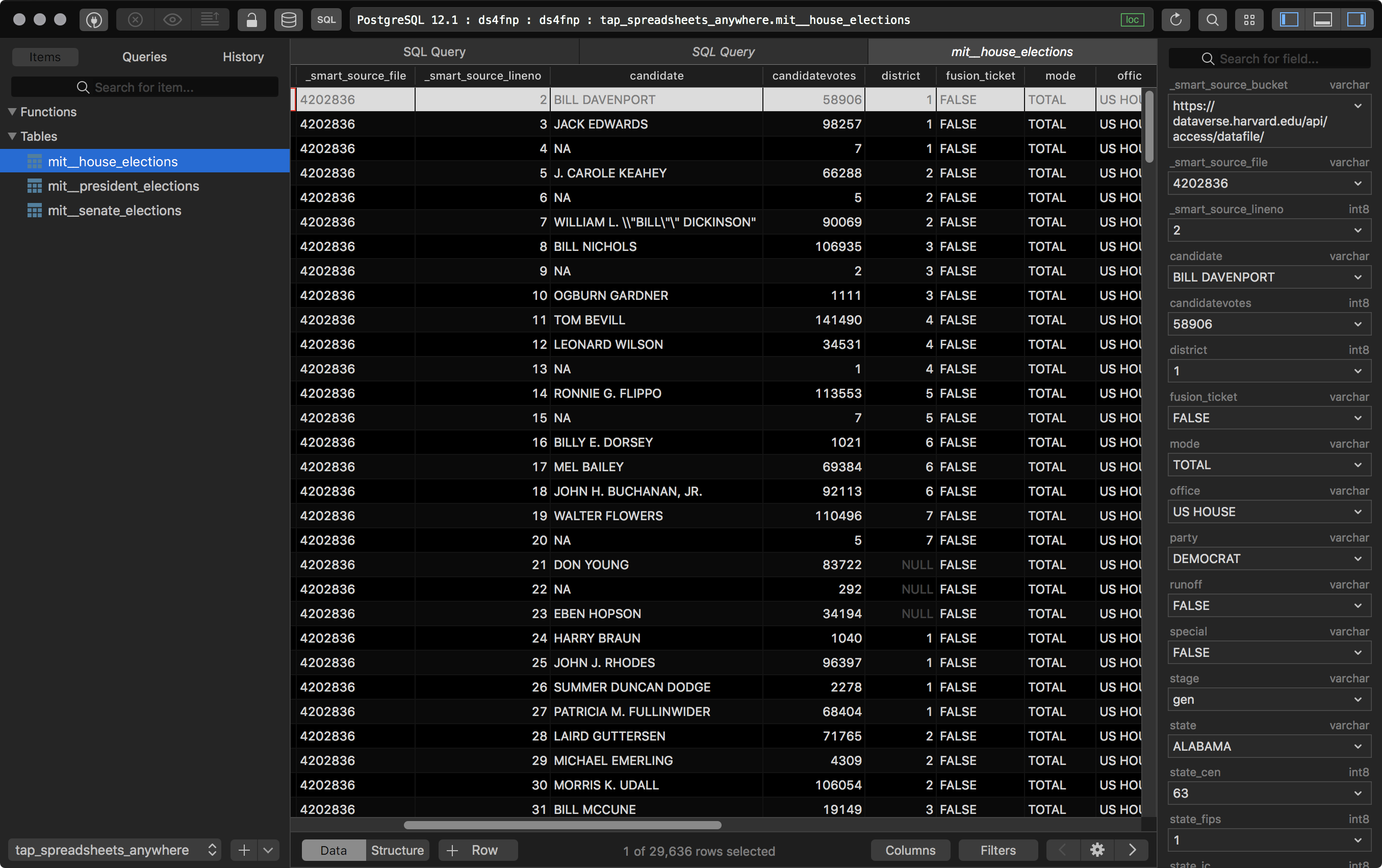
Great! We now have some raw data loaded into our database. We call this “raw” data because it contains many imperfections and uncertain quality, and ultimately we wish to refine it into more immediately useful products. The whole crude oil pipeline analogy works pretty well here. This is where transformation comes in. Some examples of the types of issues we would want to handle through data transformations:
All of the string fields in the
mit__house_electionstable are all capitalized, while in the other tables they are not. We should be consistent with capitalization.Some fields use “Firstname Lastname” while others use “Lastname, Firstname”. We should be consistent with name formats.
There are lots of metadata fields that we probably don’t care about during analysis. We can filter these out.
These election results are at a very low level of granularity, whereas we probably want to work with numbers aggregated at some higher level.
However, we’re going to handle transformations in the next step. There is actually value in maintaining our raw data as originally loaded, and treating transformations as derivatives of that raw data. Doing so helps us preserve the provenance of the data, an auditable historical record of the data in its purest collected form. It also allows us to revisit and modify our transformation tasks, which we could not do if we did not preserve the original raw data.
As I mentioned earlier, Meltano can actually incorporate dbt as a transformation layer in its own project configurations, but for now we’re going to step through dbt ourselves.
Transforming and modeling data with dbt#
dbt stands for “data build tool”. It is an open source project that provides a development environment for defining and managing analytics workflows in your data warehouse. While Singer (via Meltano) loads data into a database from one or more external sources, dbt transforms data into a new table from one or more existing tables (for example, raw data tables). This is accomplished by defining data models with basic SQL queries that utilize the Jinja templating system to dynamically reference other tables. If you have ever created web apps in frameworks like Flask where you programmatically populate content templated HTML, this does something very similar for SQL. When you run dbt, all of these templated queries and metadata are compiled into table/view definitions that are executed upon our target data warehouse. Take a moment to read more here.
Setting up dbt#
Setting up dbt is very similar to that of Meltano. We install from pip and create a new project with the dbt CLI.
cd ..                   # go back to the ds4fnp base path

pip3 install dbt        # install dbt
dbt init dbt            # create a new dbt project called 'dbt'
cd dbt                  #
We now have a fresh project skeleton, including several subdirectories and a dbt_project.yml config file which is analogous to the the meltano.yml config file. Very briefly, a dbt project consists of the following components:
sources are references to existing locations in our data warehouse where our loading processes deposit raw data. These are defined under the
modelsdirectory.models are templated queries which define selections and transformations that dbt will materialize as new tables/views in our data warehouse. Models may select from sources, or from other models. These are also defined under the
modelsdirectory.datais a directory that contains flat files in CSV format that dbt will automatically load into our data warehouse; this is useful for small immutable lookup tables.macroscontains functions which can be used by the templating engine when defining queries. We won’t get into macros too much here, but they provide the real power behind dbt.analysisqueries are similar to models except that dbt only compiles them into rendered SQL without executing them on the data warehouse. I find these useful for testing new ideas for queries without incorporating them into my overall data model, as well as pre-generating queries that can be used in downstream analyses and by BI platforms.docscontains a complete static documentation website generated by dbt. This is a really awesome feature of dbt, and is key to making your data warehouse accessible to colleagues.testsoffer a way to apply concepts from unit testing to the design of your project.snapshotsoffer a way to capture and preserve a historical record of sources that do not maintain their own history.targetis where dbt writes the compiled queries prior to execution against the target data warehouse.
For the most part we will only touch on a few of these components; namely sources and models.
We also need to configure a profiles.yml file, which will contain our database credentials and is by default located outside of the project directory under ~/.dbt/profiles.yml. I recommend reading the documentation on profile configuration.
You can configure multiple profiles, easily allowing you to then deploy your dbt project against multiple targets. For examples, you can deploy to your local postgres database for development purposes, and then deploy to BigQuery as your production data warehouse. Here’s an example profiles.yml to get us started:
# For more information on how to configure this file, please see:
# https://docs.getdbt.com/docs/profile

ds4fnp:
  outputs:
    local:
      type: postgres
      host: 127.0.0.1
      user: ds4fnp
      pass: ds4fnp
      port: 5432
      dbname: ds4fnp
      schema: public
  target: local
With our profile setup, the next thing we’ll do is turn to the project configuration. There are basically three different files we will be working with in a dbt project:
dbt_project.yml- This file informs dbt of the structure of the project, as well as a few general configuration options.schema.yml- Data models are defined through a directory structure of yaml and sql files. Theschema.ymlfiles enumerate and describe the metadata about each model.*.sql- Each model is then defined by a jinja templated SQL file. These will look fairly similar to most SQL files you may have seen, except that direct references to database objects will be replaced by macros used by the templating engine.
Rather than walk through designing an entire project configuration step by step, let’s instead look at a complete configuration. I will leave a basic overview of the dbt_project.yml file to the formal documentation.
# Name your project! Project names should contain only lowercase characters
# and underscores. A good package name should reflect your organization's
# name or the intended use of these models
name: 'ds4fnp'
version: '1.0.0'
config-version: 2

# This setting configures which "profile" dbt uses for this project.
profile: 'ds4fnp'

# These configurations specify where dbt should look for different types of files.
# The `source-paths` config, for example, states that models in this project can be
# found in the "models/" directory. You probably won't need to change these!
source-paths: ["models"]
analysis-paths: ["analysis"]
test-paths: ["tests"]
data-paths: ["data"]
macro-paths: ["macros"]
snapshot-paths: ["snapshots"]

target-path: "target"  # directory which will store compiled SQL files
clean-targets:         # directories to be removed by `dbt clean`
    - "target"
    - "dbt_modules"


# Configuring models
# Full documentation: https://docs.getdbt.com/docs/configuring-models

# In this example config, we tell dbt to build all models in the example/ directory
# as tables. These settings can be overridden in the individual model files
# using the `{{ config(...) }}` macro.
models:
  ds4fnp:
    staging:
        +schema: staging
        +materialized: view
    # marts:
    elections:
        +schema: elections
        +materialized: view
Except for a couple edits, this is pretty much the stock configuration file that dbt generated for us during initialization. The main things we changed are pointing profile: to the profile we created above, and everything under the models: section. There are several ways to structure your data models, but we’ll keep things fairly simple here. I have defined just two schemas:
stagingwill contain references to our data sources.electionswill contain the transformation models that we will use downstream.
Defining sources and staging tables#
First let’s define our staging schema in models/staging/schema.yml. From Meltano, we loaded three different sources into our warehouse (House, Senate, and Presidential election results).
version: 2

sources:
  - name: mit
    loader: meltano
    database: ds4fnp
    schema: tap_spreadsheets_anywhere
    tables:
      - name: mit__house_elections
        description: MIT house election data
      - name: mit__senate_elections
        description: MIT senate election data
      - name: mit__president_elections
        description: The data file `1976-2016-president` contains constituency (state-level) returns for elections to the U.S. presidency from 1976 to 2016.  The data source is the document "[Statistics of the Congressional Election](http://history.house.gov/Institution/Election-Statistics/Election-Statistics/)," published biennially by the Clerk of the U.S. House of Representatives.
        columns:
          - name: candidate
            description: name of the candidate
          - name: candidatevotes
            description: votes received by this candidate for this particular party
          - name: district
            description: None
        ...
models:
  - name: stg_us_house_election_results
    description: US House election results
  - name: stg_us_senate_election_results
    description: US Senate election results
  - name: stg_us_president_election_results
    description: US President election results
In this file, we define the locations to our source tables under sources:, but we also define a corresponding set of “staging” models under models:. The value of each name: field must then correspond to a .sql file which we will also create. The reason we define staging models for each data source is that we may want to use the same source in multiple data models, but we don’t necessarily want to define the same filtering and data cleaning in every single instance. With a staging model, we can define those transformations one time and in one single place so that any modifications to that data source can be reflected in every downstream model that references it. The schema.yml file also allows us to describe and document the fields in our tables, which will come in handy later.
Defining data models#
For the model definitions, I’ll just use the House elections as an example, as the other two will look similar and the full code is available from the Github repository mentioned earlier. We will define the staging model for House election results in models/staging/stg_us_house_election_results.sql:
select
    to_date(year::VARCHAR, 'YYYY') as year,
    INITCAP(candidate) as candidate,
    INITCAP(party) as party,
    INITCAP(state) as state,
    state_po,
    COALESCE(district, '1') as district,
    candidatevotes::INTEGER as candidate_votes,
    totalvotes as total_votes,
	ROUND(candidatevotes::numeric / totalvotes::numeric * 100, 2) as vote_pct
from {{ source('mit','mit__house_elections') }}
where writein::BOOLEAN is False
As we can see from this staging model, the templated SQL in dbt mostly resembles regular SQL, except that we use a {{ source() }} macro in the from clause of the query. When dbt runs, it will populate the macro with the appropriate information from the project configuration. In this staging model, we are basically selecting the source table as-is, except that we limit the fields returned and perform some transformations to a few of them. For example:
We have converted the
datefield to an actual date stamp type.We have corrected the all-caps strings in many fields with the
INITCAP()function.We have interpolated some missing values in the
districtcolumn.
Just to name a few. We then repeat this for the Senate and President election data sources. Now that we have defined our sources and staging models, we can begin designing the data models we plan to use in our future analyses and in Superset. Wheres the raw data provides election results for every single candidate (including write-ins, minor parties, etc) and each state/district, let’s work towards summarizing the results at the party level. For these models we will create a new schema under models/elections/schema.yml:
version: 2

models:
  - name: us_house_party_seats
    description: Seats in the US House of Representatives by party.
  - name: us_senate_party_seats
    description: Seats in the US Senate by party.
  - name: us_president_popular_vote
    description: Popular vote in US presidential elections by party.
This should look similar to the staging models we defined above. To summarize the House results, let’s define a data model query that ranks and filters the candidates by votes received, and then finally aggregates the number of seats won by each party for each election year.
WITH
sub1 AS (
    SELECT
        *,
        rank() OVER (PARTITION BY year,
        state,
        district ORDER BY candidate_votes DESC) AS rank
    FROM {{ ref('stg_us_house_election_results') }}
),
sub2 AS (
    SELECT
        *,
        rank = 1 AS winner
    FROM sub1
)

SELECT
	year,
	party,
	count(*) as seats
FROM sub2
WHERE winner = True
GROUP BY year, party
Our query looks fairly similar to that used in the staging model, with the main difference being the use of the {{ ref() }} macro instead of the {{ source() }} macro. The other queries can be found in the Github repository.
Running dbt#
After we have our project configured, we can now run dbt! Note that in practice you probably want to run the project fairly often as you go along to validate your work. To do so, we simply run dbt run from the command line. I’ll include the terminal output in the code snippet here:
dbt run

Running with dbt=0.18.1
Found 6 models, 0 tests, 0 snapshots, 1 analysis, 138 macros, 0 operations, 0 seed files, 3 sources

14:08:49 | Concurrency: 1 threads (target='local')
14:08:49 |
14:08:49 | 1 of 5 START view model dbt_staging.stg_us_house_election_results.... [RUN]
14:08:49 | 1 of 5 OK created view model dbt_staging.stg_us_house_election_results [CREATE VIEW in 0.23s]
14:08:49 | 2 of 5 START view model dbt_staging.stg_us_senate_election_results... [RUN]
14:08:49 | 2 of 5 OK created view model dbt_staging.stg_us_senate_election_results [CREATE VIEW in 0.08s]
14:08:49 | 3 of 5 START view model dbt_staging.stg_us_president_election_results [RUN]
14:08:49 | 3 of 5 OK created view model dbt_staging.stg_us_president_election_results [CREATE VIEW in 0.08s]
14:08:49 | 4 of 5 START view model dbt_elections.us_house_party_seats........... [RUN]
14:08:50 | 4 of 5 OK created view model dbt_elections.us_house_party_seats...... [CREATE VIEW in 0.09s]
14:08:50 | 5 of 5 START view model dbt_elections.us_senate_party_seats.......... [RUN]
14:08:50 | 5 of 5 OK created view model dbt_elections.us_senate_party_seats..... [CREATE VIEW in 0.07s]
14:08:50 |
14:08:50 | Finished running 5 view models in 1.26s.

Completed successfully

Done. PASS=5 WARN=0 ERROR=0 SKIP=0 TOTAL=5
Awesome, our project compiled and ran successfully! You can follow the progress as dbt runs and it will often provide informative diagnostics if something goes wrong.Before we peer into our data warehouse to see everything dbt generated, let’s quickly go over generating dbt’s docs. We do this with just two more commands:
dbt docs generate
dbt docs serve
This will generate your data warehouse’s documentation and spin up a temporary webserver so you can view it. Take a minute to explore the generated site in your browser.
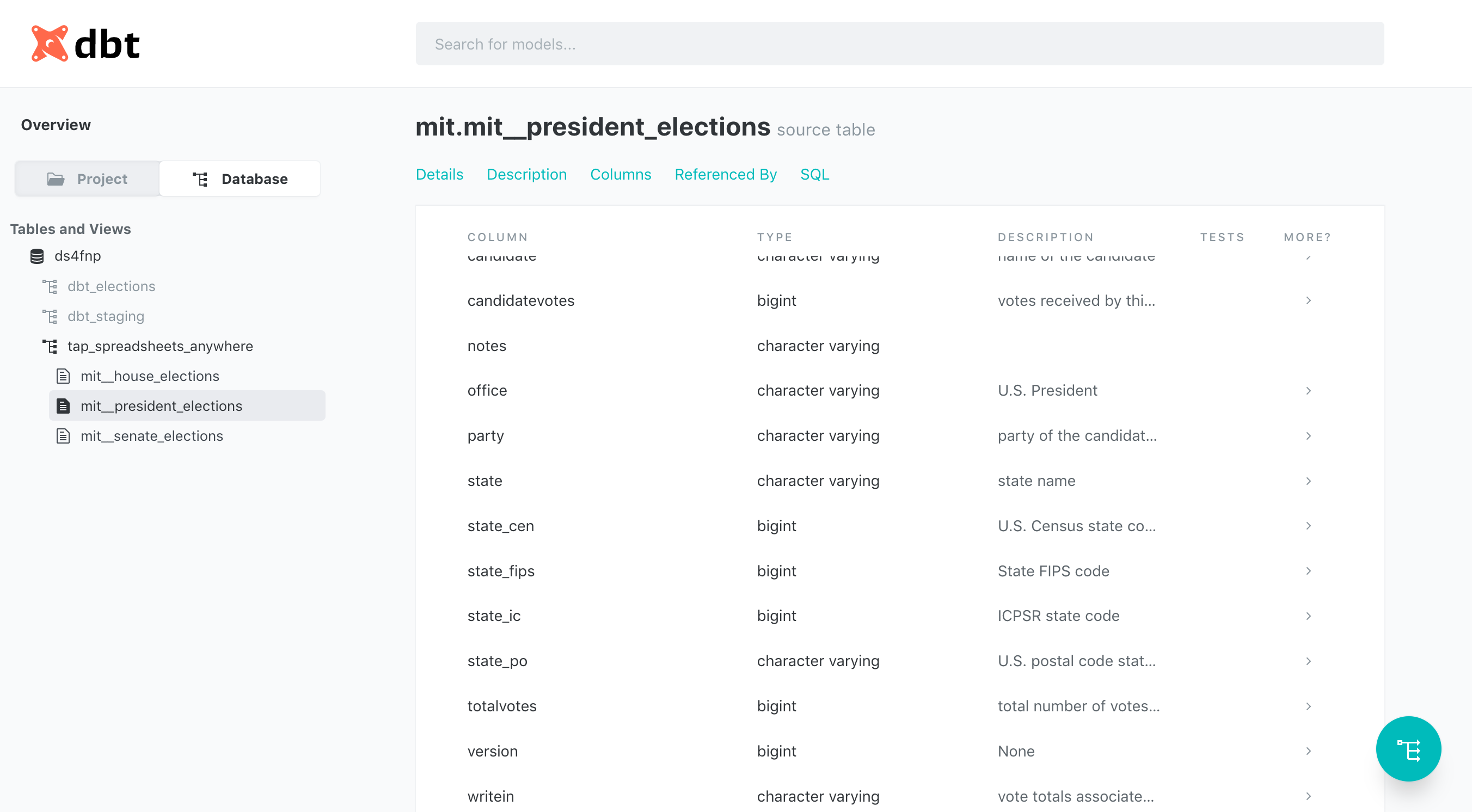
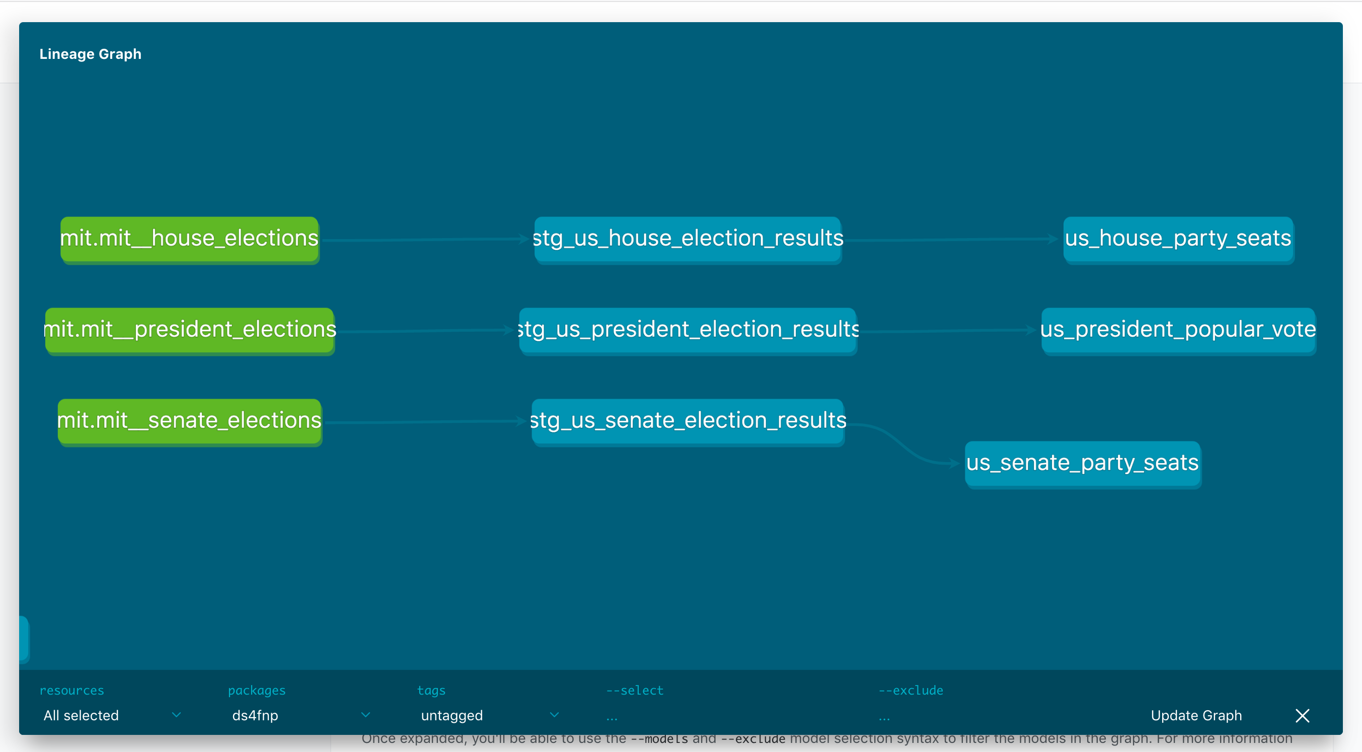
One of the great features with dbt is the graph on the right side of the site that allows you to visualize the relationships between your various views and tables. Note that unlike ERD (Entity Relationship Diagrams) that you may have seen elsewhere, the relationships between tables here are of lineage; ie, which tables are the sources of other tables. As projects grow in complexity, these diagrams and the auto-generated documentation in general can become highly valuable.
At this point you can also examine the tables you have generated in your local postgres data warehouse. We will take a more directed look at them in the next section.
Analyzing and visualizing data with Superset#
At last we are ready to do something with our newly populated data warehouse. Typically any analytics project is going to have some sort of BI layer with interactive data visualizations being dynamically updated with the data from our warehouse. Of course, in this tutorial we are intentionally using an infrequently updated source of data (US elections only occur every two years). None the less, we can setup Apache Superset to demonstrate how one goes about this general task.
Once again we will run a bunch of commands at the terminal:
pip3 install apache-superset                # install superset
superset db upgrade                         # initialize superset's db
superset fab create-admin                   # create an admin user
superset init                               # set a bunch of defaults
superset run -p 8088 --with-threads --reload --debugger     # run it!
A few of these steps may involve some interaction, after which you should have a running instance of Superset that you can reach from your browser at http://localhost:8088. At this point I would also recommend taking a quick skim through Superset’s documentation. Because the rest of this tutorial is away from the command line, I’ll first list the steps towards creating a dashboard in Superset, and then we’ll walk through them. If you have used commercial BI tools like Tableau or Looker, this will look very similar.
Configure a data sourceCreate datasetsCreate chartsCreate dashboards
If you want to skip right to the finished product, you can import the data and dashboard configurations that I’ve exported to the Github repository under the superset directory:
superset import-datasources -p datasources.yml
superset import-dashboards -p dashboards.json
Configuring a data source#
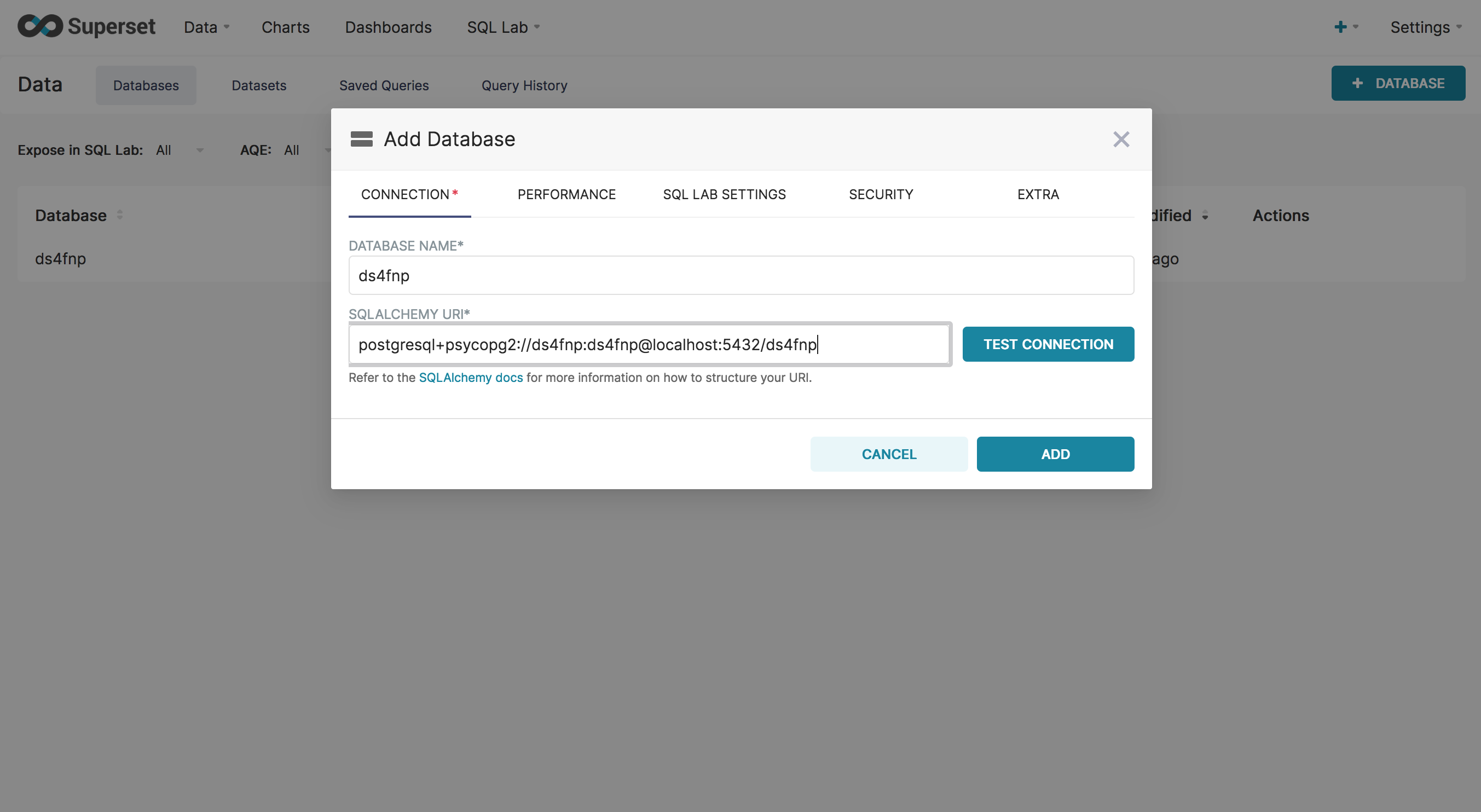
We only need to establish a connection to our warehouse as data source. You can add new connections by going to “Databases” under the “Data” menu. Superset uses SQLAlchemy to manage database connections, so your connection string will look like this: postgresql+psycopg2://ds4fnp:ds4fnp@localhost:5432/ds4fnp
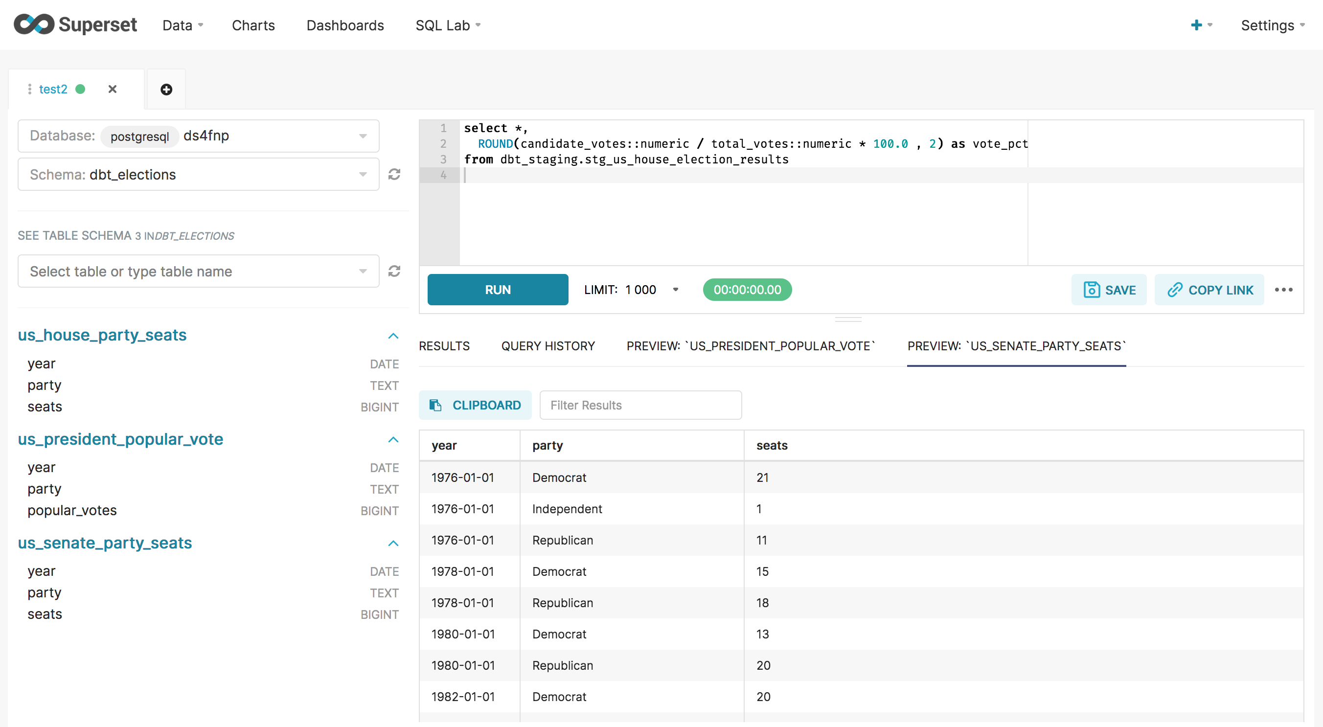
Before we get into data visualization, it’s worth pointing out that Superset has a handy built-in SQL client called “SQL Lab”. Once you have added a data source, you can use the SQL Lab to browser database tables and run SQL queries. This really useful for running ad-hoc analyses, as well as aiding development in Meltano and dbt.
Creating datasets#
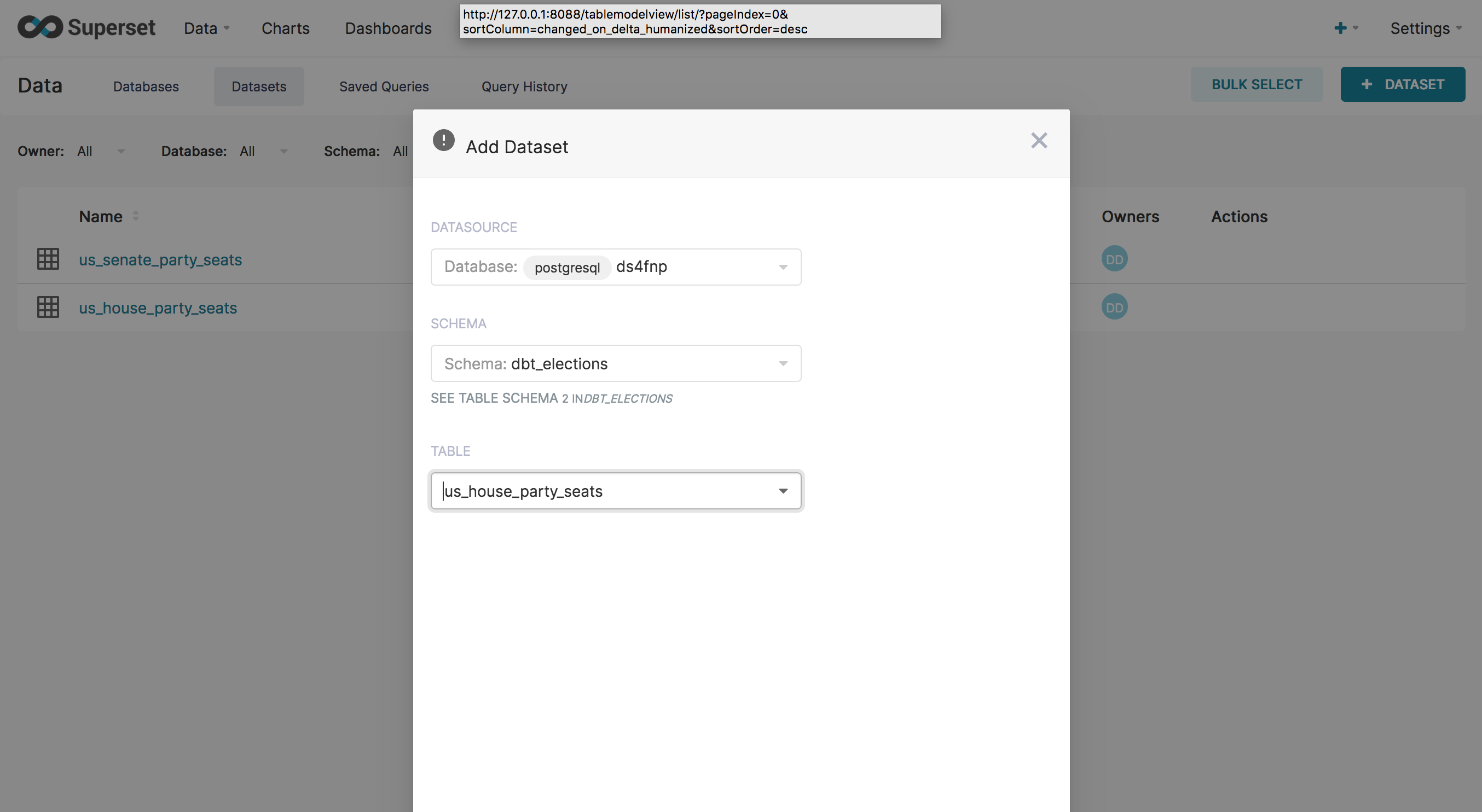
Also under the “Data” menu is “Datasets”, which are typically going to be tables selected from your warehouse. To create one, you select the database, schema, and table, and click save.
Creating charts#
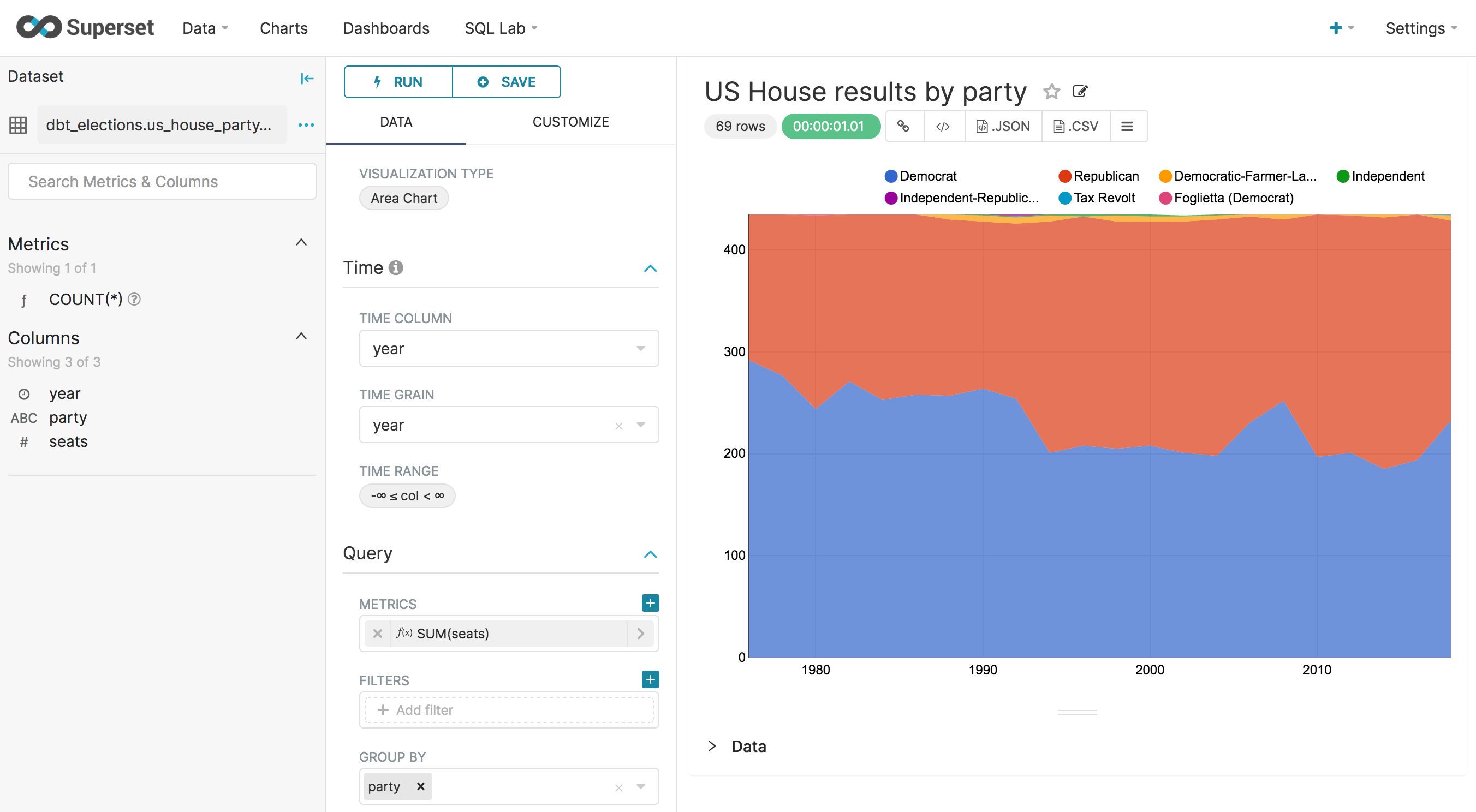
Charts are the heart of Superset. Creating one involves specifying which dataset to use, and then mapping various visual aesthetics to fields in your dataset. We will create a very simple example here:
Create a new chart.
Select “dbt_elections.us_house_party_seats” as the dataset, and “Area Chart” as the chart type.
Select
yearas the time column, as well as the time grain.Set the time range to “No Filter”.
Under metrics, select
seatsas the column andSUMas the aggregate.Select
partyto group by.
I also changed the color scheme under Customize to “Google Category 10c”, mostly to map the Democratic party to blue and the Republican party to red.
Repeat this process to create similar charts for the Senate and President election results.
Note: Yes, I realize that democrats are red and republicans are blue in the Presidential election chart. To address this, we would probably want to create an additional standardized party field in our tables in order to control how groupings and orderings work.
Creating dashboards#
Dashboards in Superset provide a canvas for assembling charts and other artifacts into a single convenient page that users can view and interact with. Superset makes it very easy to create a new dashboard and drag-and-drop charts onto the canvas. Check out Preset.io’s documentation on Superset dashboards for further information on how to customize all of the various dashboard features.
For this tutorial, I simply created a fresh dashboard and dragged each chart we just created onto it.
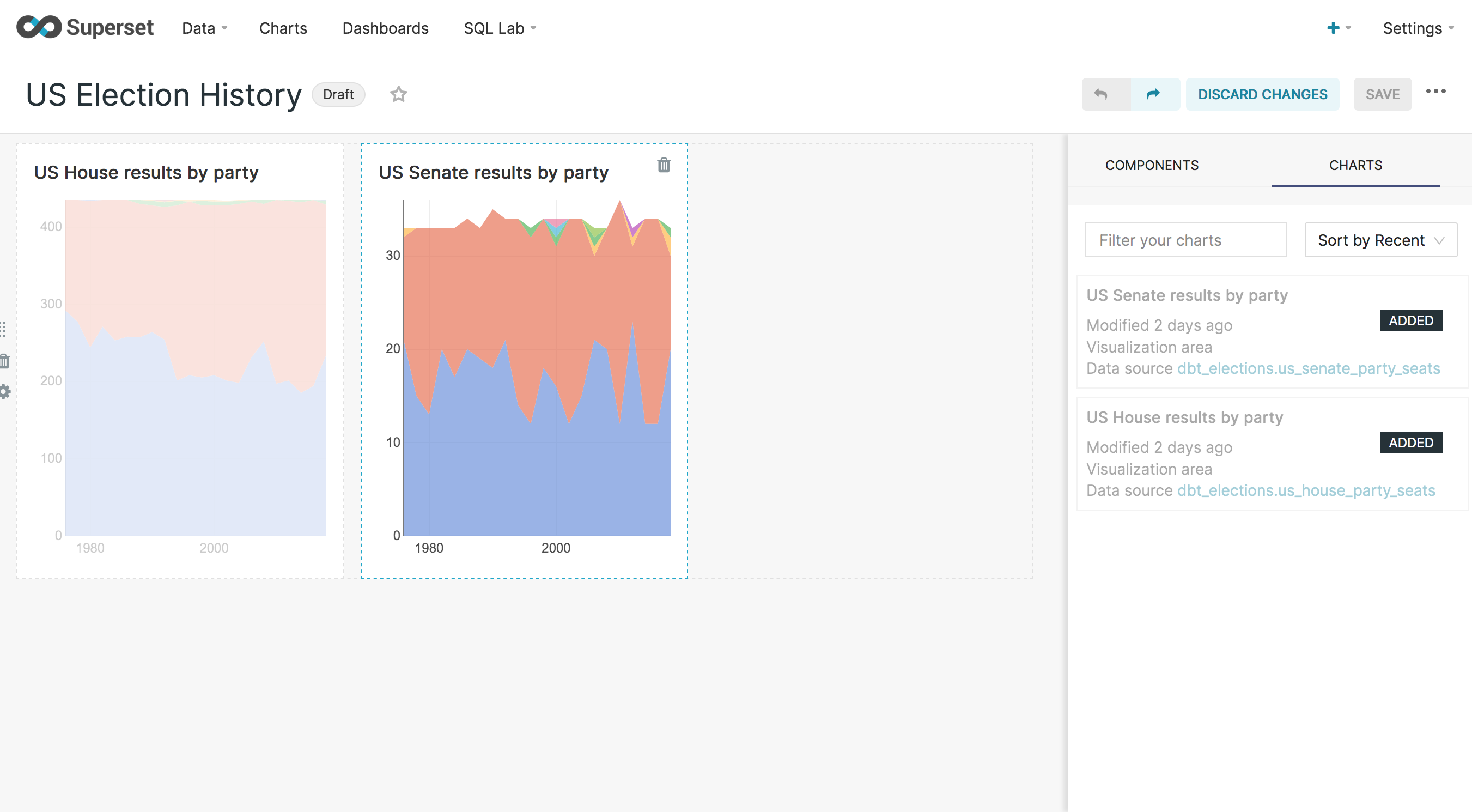
Once you have your dashboard looking how you want it to, just save it and click on the “Draft” toggle to set the dashboard as published.
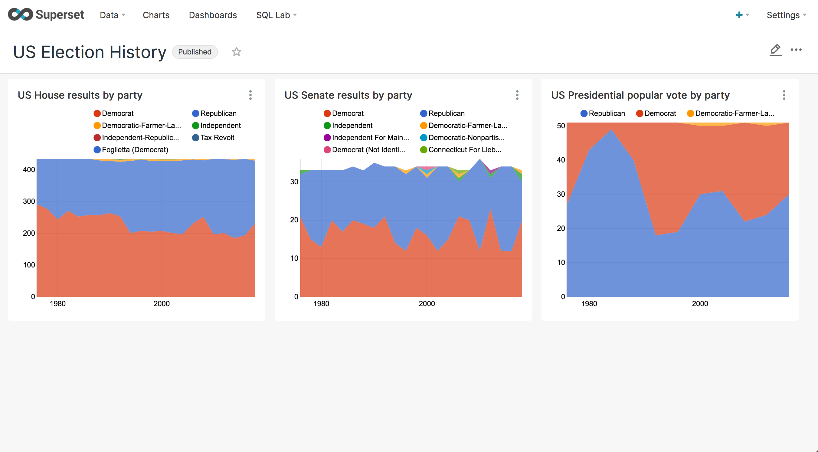
This looks like a pretty good start! From here you can experiment with creating more charts and dashboards. You may also want to go back to your data model and create additional tables/views that can power other types of charts. If you are feeling especially bold, you may even want to try adding additional loaders in Meltano and combining multiple data sources in your dbt project.
Wrapping up#
To recap, in this tutorial we have:
Installed and configured each piece of the DS4FNP stack.
Created a postgres database as our local development warehouse.
Loaded our warehouse with data we extracted from external sources using Meltano.
Transformed our raw data into refined data models using dbt.
Created visualizations from our data model in Superset.
Hopefully you should now have a good grasp of the technologies in the stack and how they come together to create a modern data analytics system. What we have covered is by no means the extent of what is involved in developing a full production quality system, but it does establish a foundation to build from.
We just used a simple postgres instance running on our local machine for this tutorial, and doing so is indeed perfecttly valid for local development purposes, but at some point we want to utilize a scalable cloud based warehouse like BigQuery or Snowflake. Fortunately the transition from local development warehouse to cloud production warehouse is pretty easy with this stack. Assuming we have a provisioned instance running somewhere, we would simply add its connection and credentials to our project configurations in Meltano and dbt. These tools make it very easy to switch between deployment targets.
For a real production environment, you probably also don’t want to run these tools from your local machine. Instead you would want to execute your pipelines using cloud based computing. You could roll your own solution by hand, but fortunately there are existing cloud platforms that are simple to use. For example, the creators of dbt offer dbt Cloud as a hosted service that “comes equipped with turnkey support for scheduling jobs, CI/CD, serving documentation, monitoring & alerting, and an Integrated Developer Environment (IDE).”
Speaking of CI/CD, one of the benefits of defining your data warehouse through configuration and code is that you can manage those files with a version control system (like git) and treat the execution of your pipelines as a similar to a build process with your warehouse as the build target. If you don’t understand what any of that means right now, we’ll touch on some DevOps topics in later tutorials.
While your data pipelines can run only when needed (either triggered or), you will most likely want to have Superset running continuously so that you can acccess it as needed. In a production environment, this is something you would want to deploy as a managed web service. Similar to how dbt Cloud offers a hosted service for running dbt, Preset.io offers a hosted service for running Superset.
The examples we used throughout this tutorial were somewhat oversimplified in order to present a broad overview of the entire stack and process, but subsequent tutorials will drill further down into specific aspects and include additional topics. Some of these will include configuring CI/CD workflows, more advanced data source extraction, orchestration of workflows with Airflow, designing metrics, and working with cloud warehouses.
I hope you found this tutorial useful!
